Robust Joint Modelling Framework
Joint modelling of longitudinal time-to-event outcomes typically combines a linear mixed-effects model for repeated measures and a Cox model with time-varying frailty for time-to-event outcome (Asar et al., 2015). Typical distributional assumption is that random-effects and measurement error terms in mixed-effects model are Gaussian. However, this assumption might be restricive for real-life problems, where it is quite likely to have
subjects who do not conform the population averaged trends (they are examples of outliers in the random-effects), and
subjects who has a few observations that are quite different compared to the rest of the observations for subjects’ own collection of measurements (they are examples of outliers in measurement error).
Gaussian distribution would not give appropriate weights to the outliers, hence inference might be biased and inefficient, and personalised predictions might be misleading. A natural approach would be to replace the Gaussian assumption with t distribution. Technical details of joint models with t distributions, and associated inferential methods are skipped here, and interested reader is referred to Asar, Fournier and Dantan (2019).
Implementation
We describe the
R package robjm to implement the
joint models with Gaussian and t distributed random-effects and error terms,
and subsequently to obtain personalised dynamic predictions.
For illustration, we will use the
AIDS data-set (first 250 subjects only).
Note that the biomarker of interest is the CD4 cell counts, and the
survival event is death.
robjm is still under development, hence is currently only available from Github.
To install robjm from Github and load into the working environment,
use the following lines:
devtools::install_github("ozgurasarstat/robjm", quiet = TRUE)
suppressMessages(library(robjm))
AIDS data-set can be loaded and prepared for analysis using
data(aids)
data(aids.id)

aids$drug2 <- ifelse(aids$drug == "ddC", 0, 1)
aids.id$drug2 <- ifelse(aids.id$drug == "ddC", 0, 1)

idlist <- aids.id$patient

long_data <- aids[aids$patient %in% idlist[1:250], ]
surv_data <- aids.id[aids.id$patient %in% idlist[1:250], ]
Below, we first fit the joint model with Gaussian random effects and Gaussian error terms, and then Gaussian random effects and t distributed error terms.
fit_nor_nor <- fit_jm(fixed_long = CD4 ~ obstime,
                      random_long = ~ obstime,
                      fixed_surv = cbind(Time, death) ~ drug2,
                      data_long = long_data,
                      data_surv = surv_data,
                      id_long = "patient",
                      id_surv = "patient",
                      model = "nor_nor",
                      timeVar = "obstime",
                      bh = "weibull",
                      chains = 4,
                      cores = 4,
                      iter = 2000,
                      warmup = 1000,
                      control = list(adapt_delta = 0.9)
                      )

fit_nor_t <- fit_jm(fixed_long = CD4 ~ obstime,
                  random_long = ~ obstime,
                  fixed_surv = cbind(Time, death) ~ drug2,
                  data_long = long_data,
                  data_surv = surv_data,
                  id_long = "patient",
                  id_surv = "patient",
                  model = "nor_t_mod3",
                  timeVar = "obstime",
                  bh = "weibull",
                  chains = 4,
                  cores = 4,
                  iter = 2000,
                  warmup = 1000,
                  control = list(adapt_delta = 0.9)
                  )
The results can be summarised by
print(fit_nor_nor$res,
      pars = c("alpha", "Sigma", "sigmasq", "log_lambda",
               "log_nu", "omega", "eta"))
## Inference for Stan model: cc3bb0e249a9f8cb9af6f1735fffcd05.
## 4 chains, each with iter=2000; warmup=1000; thin=1;
## post-warmup draws per chain=1000, total post-warmup draws=4000.
##
##             mean se_mean   sd  2.5%   25%   50%   75% 97.5% n_eff Rhat
## alpha[1]    7.63    0.02 0.30  7.03  7.43  7.63  7.83  8.24   353 1.01
## alpha[2]   -0.19    0.00 0.02 -0.24 -0.21 -0.19 -0.18 -0.15  1127 1.00
## Sigma[1,1] 22.34    0.04 2.26 18.28 20.74 22.19 23.74 27.18  3004 1.00
## Sigma[1,2]  0.09    0.00 0.11 -0.12  0.02  0.09  0.16  0.30  1048 1.00
## Sigma[2,1]  0.09    0.00 0.11 -0.12  0.02  0.09  0.16  0.30  1048 1.00
## Sigma[2,2]  0.04    0.00 0.01  0.02  0.03  0.04  0.05  0.06   186 1.01
## sigmasq     3.62    0.01 0.29  3.12  3.41  3.59  3.79  4.25   473 1.01
## log_lambda -2.89    0.01 0.49 -3.83 -3.22 -2.88 -2.56 -1.93  2189 1.00
## log_nu      0.27    0.00 0.12  0.02  0.19  0.27  0.35  0.49  2081 1.00
## omega[1]    0.52    0.00 0.26  0.02  0.34  0.52  0.69  1.04  3299 1.00
## eta        -0.49    0.00 0.08 -0.68 -0.54 -0.48 -0.43 -0.35  1326 1.00
##
## Samples were drawn using NUTS(diag_e) at Wed Jul 24 13:06:40 2019.
## For each parameter, n_eff is a crude measure of effective sample size,
## and Rhat is the potential scale reduction factor on split chains (at
## convergence, Rhat=1).
print(fit_nor_t$res,
      pars = c("alpha", "Sigma", "sigmasq", "delta",
               "log_lambda", "log_nu", "omega", "eta"))
## Inference for Stan model: 3350d3e47d14b2f21179f624bafbbcb5.
## 4 chains, each with iter=2000; warmup=1000; thin=1;
## post-warmup draws per chain=1000, total post-warmup draws=4000.
##
##             mean se_mean   sd  2.5%   25%   50%   75% 97.5% n_eff Rhat
## alpha[1]    7.62    0.02 0.32  6.98  7.41  7.62  7.83  8.23   171 1.01
## alpha[2]   -0.19    0.00 0.02 -0.23 -0.21 -0.19 -0.18 -0.16  1208 1.00
## Sigma[1,1] 22.87    0.04 2.25 18.86 21.30 22.75 24.32 27.64  3420 1.00
## Sigma[1,2]  0.08    0.00 0.09 -0.09  0.02  0.08  0.14  0.26   985 1.00
## Sigma[2,1]  0.08    0.00 0.09 -0.09  0.02  0.08  0.14  0.26   985 1.00
## Sigma[2,2]  0.03    0.00 0.01  0.01  0.02  0.03  0.03  0.04   277 1.01
## sigmasq     1.41    0.02 0.23  1.01  1.25  1.39  1.56  1.92   183 1.01
## delta       3.10    0.05 0.56  2.25  2.71  3.02  3.40  4.40   153 1.01
## log_lambda -2.97    0.01 0.47 -3.90 -3.27 -2.96 -2.65 -2.03  2555 1.00
## log_nu      0.27    0.00 0.11  0.04  0.19  0.27  0.35  0.49  2531 1.00
## omega[1]    0.48    0.00 0.23  0.03  0.32  0.48  0.64  0.93  4258 1.00
## eta        -0.45    0.00 0.07 -0.59 -0.49 -0.45 -0.40 -0.32  2063 1.00
##
## Samples were drawn using NUTS(diag_e) at Wed Jul 24 13:19:32 2019.
## For each parameter, n_eff is a crude measure of effective sample size,
## and Rhat is the potential scale reduction factor on split chains (at
## convergence, Rhat=1).
Traceplots of the MCMC samples can be visualised by
traceplot(fit_nor_nor$res,
          pars = c("alpha", "Sigma", "sigmasq", "log_lambda",
                   "log_nu", "omega", "eta"),
          inc_warmup = FALSE)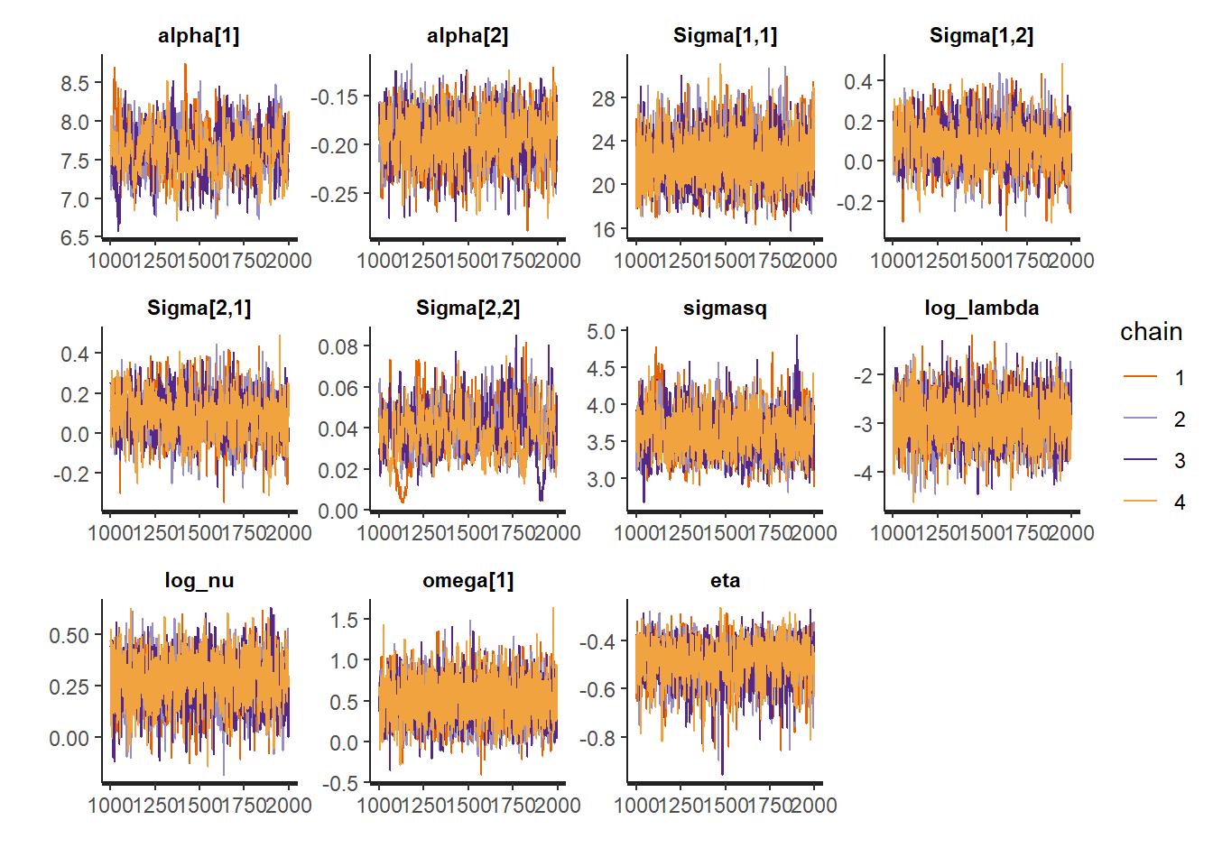
traceplot(fit_nor_t$res,
pars = c("alpha", "Sigma", "sigmasq", "delta",
"log_lambda", "log_nu", "omega", "eta"),
inc_warmup = FALSE)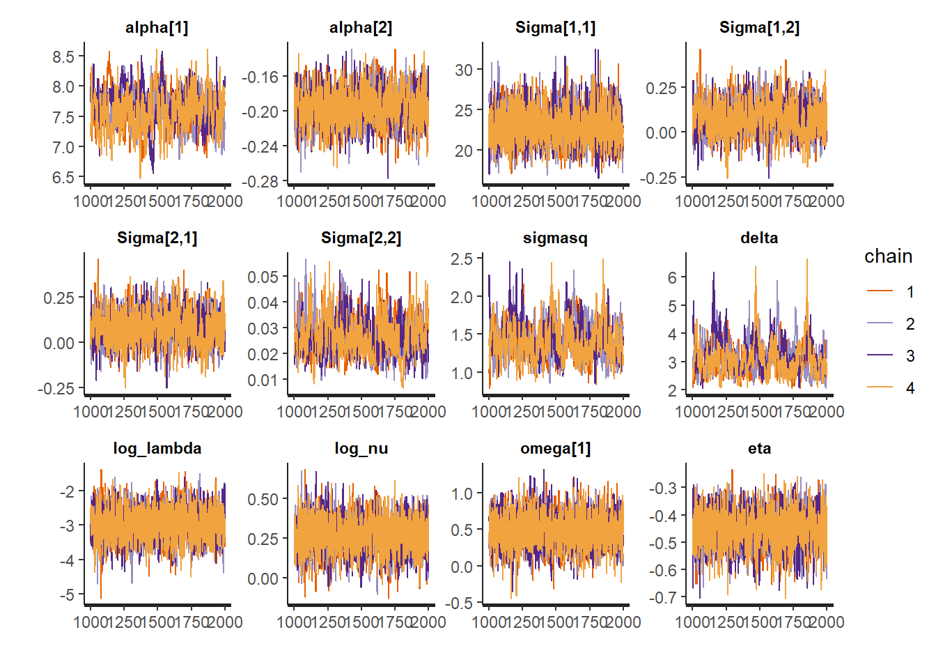 1-, 2-, 3-, 4- and 5-year survival probabilities for a new subject,
say 251th subject, can be obtained by
1-, 2-, 3-, 4- and 5-year survival probabilities for a new subject,
say 251th subject, can be obtained by
newdata <- dplyr::filter(aids, patient == idlist[251])

fore_nor_nor <- predSurv_jm(object = fit_nor_nor,
                            newdata = newdata,
                            forecast = list(h = 5, n = 5),
                            B_control = list(nsel_b = 1, init = 0)
                            )

fore_nor_t <- predSurv_jm(object = fit_nor_t,
                          newdata = newdata,
                          forecast = list(h = 5, n = 5),
                          B_control = list(nsel_b = 1, init = 0)
                          )
The output would be displayed as a matrix by
fore_nor_nor$output
##    id  time      mean      2.5%       50%     97.5%
## 1 251 12.67 1.0000000 1.0000000 1.0000000 1.0000000
## 2 251 13.67 0.9396074 0.8058206 0.9520021 0.9898344
## 3 251 14.67 0.8738941 0.6045039 0.8982194 0.9791520
## 4 251 15.67 0.8043420 0.4122931 0.8395575 0.9676369
## 5 251 16.67 0.7328315 0.2531203 0.7752642 0.9556265
## 6 251 17.67 0.6613614 0.1302842 0.7061108 0.9423222

fore_nor_t$output
##    id  time      mean      2.5%       50%     97.5%
## 1 251 12.67 1.0000000 1.0000000 1.0000000 1.0000000
## 2 251 13.67 0.9402967 0.8618955 0.9465695 0.9813550
## 3 251 14.67 0.8761642 0.7145185 0.8889168 0.9613291
## 4 251 15.67 0.8084205 0.5648494 0.8270832 0.9393713
## 5 251 16.67 0.7382199 0.4179627 0.7618242 0.9176277
## 6 251 17.67 0.6669916 0.2906182 0.6933998 0.8940972